Views#

Views are computed DataFrames that dynamically join and transform data from multiple tables on-the-fly. Unlike persisted tables, views compute their data when accessed and can optionally be materialized to tables for performance.

JoinedTimeseriesView#

The JoinedTimeseriesView is the most commonly used view and typically the starting point for generating metrics and doing analysis. It joins primary and secondary timeseries data with the location crosswalks and optionally adds location attributes.

Understanding the Join Process#

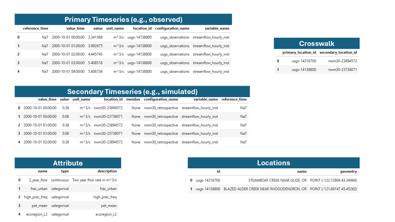
../_images/joinedTS_tutorial-1.png — Example NWM and USGS data in the TEEHR data model.#

The view brings together multiple tables:

Primary Timeseries: Observed data (e.g., USGS streamflow)
Secondary Timeseries: Simulated data (e.g., NWM forecasts)
Locations: Point geometries
Location Crosswalks: Mapping between primary and secondary location IDs
Location Attributes: Attribute values for each location

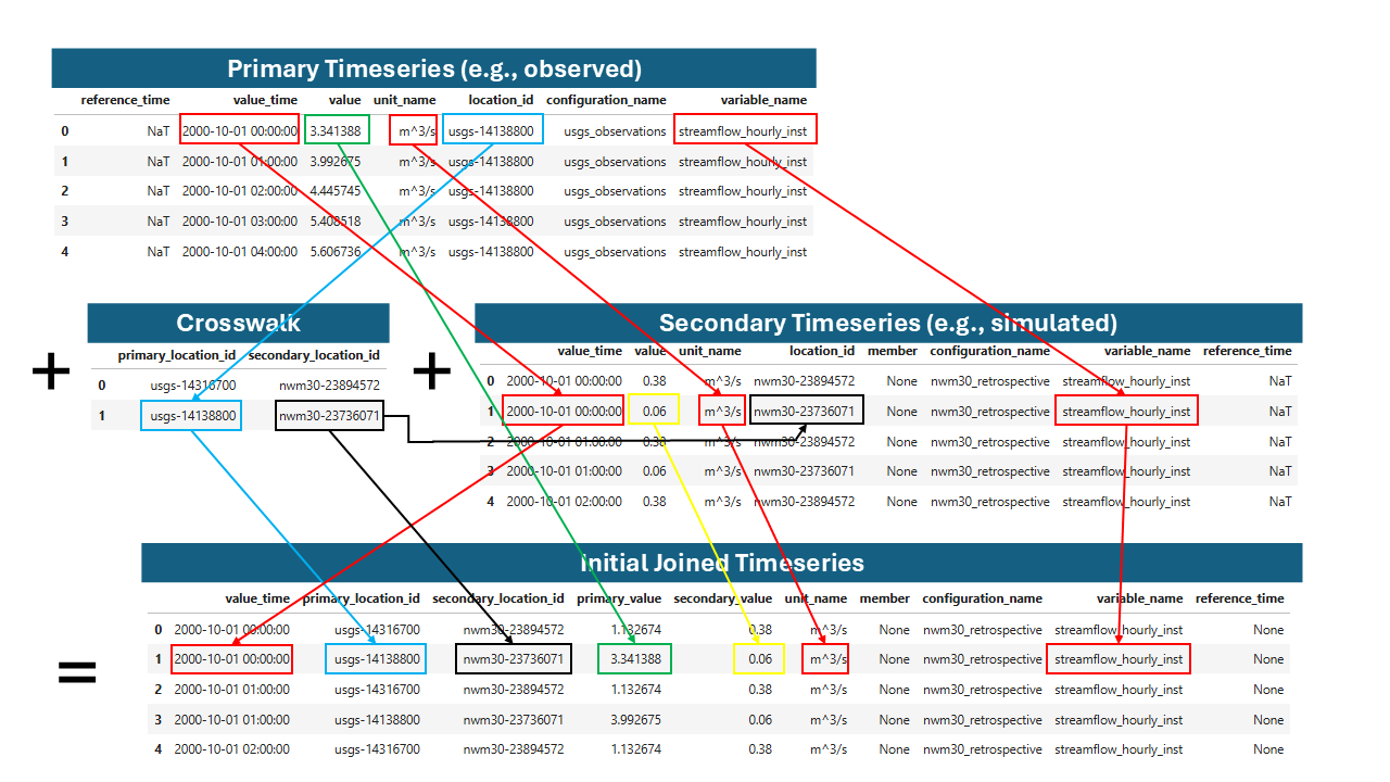
../_images/joinedTS_tutorial-2.png — Joining primary and secondary values by location, time, variable name, and unit. The variable joining has some special behavior that allows any instantaneous values to be joined to any other instantaneous values regardless of the interval, which is covered in the documentation for the view method parameters.#

The result is a unified table for analysis such as calculating metrics or generating visualizations.

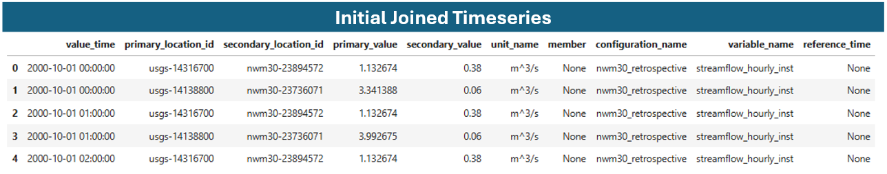
../_images/joinedTS_tutorial-3.png — Example joined timeseries table.#

Basic Usage#

Create a joined timeseries view:

import teehr

ev = teehr.LocalReadWriteEvaluation(dir_path="/path/to/evaluation")

# Basic joined view
jt = ev.joined_timeseries_view()

# View as Spark DataFrame (recommended for large datasets)
jt.to_sdf().show()

# Or convert to pandas for smaller datasets
df = jt.to_pandas()

Adding Location Attributes#

Join location attributes to the timeseries data:

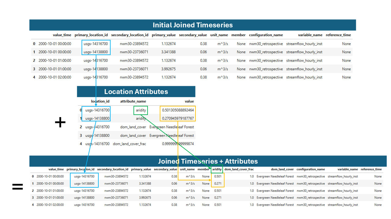
../_images/joinedTS_tutorial-5.png — Joining attributes to the joined timeseries table.#

# Add all available attributes
jt = ev.joined_timeseries_view(add_attrs=True)

# Add specific attributes only
jt = ev.joined_timeseries_view(
    add_attrs=True,
    attr_list=["drainage_area", "ecoregion"]
)

Filtering Views#

Apply SQL-style filters to narrow results:

# Filter by location pattern
jt = ev.joined_timeseries_view().filter(
    "primary_location_id LIKE 'usgs-02424000'"
)

# Filter by date range
jt = ev.joined_timeseries_view().filter(
    "value_time BETWEEN '2020-01-01' AND '2020-12-31'"
)

# Multiple filter conditions
jt = ev.joined_timeseries_view(add_attrs=True).filter("""
    primary_location_id LIKE 'usgs-02424000'
    AND CAST(drainage_area AS DOUBLE) > 100
    AND configuration_name = 'nwm30_retrospective'
""")

Materializing Views to Tables#

For repeated queries, materialize a view to an Iceberg table:

Note

Writing a view to a table is only available for users with write permissions, so LocalReadWriteEvaluation is required.

Note

Materializing a view creates a physical table with the current data. Future changes to source tables won’t affect the materialized table unless you overwrite it.

# Write view to a named table
ev.joined_timeseries_view(add_attrs=True).write("joined_with_attrs")

# Later, query the materialized table directly
df = ev.table("joined_with_attrs").aggregate(
    metrics=[DeterministicMetrics.KlingGuptaEfficiency()],
    group_by=["primary_location_id"]
).to_pandas()

Other Views#

LocationAttributesView#

Pivots the location_attributes table from long format to wide format, with each attribute as a column. This view is useful for joining location attributes to timeseries data or for other analyses that require a wide format, similar to a traditional geospatial “attributes table”.

# Pivot all attributes
la = ev.location_attributes_view()
la.to_sdf().show()

# Pivot specific attributes
la = ev.location_attributes_view(
    attr_list=["drainage_area", "percent_forest"]
)

# Filter and view
la.filter(
    "CAST(drainage_area AS DOUBLE) > 100"
).to_sdf().show()

# Materialize for reuse
ev.location_attributes_view().write("pivoted_attrs")

PrimaryTimeseriesView#

View of primary timeseries with optional location attributes:

# Basic view
pv = ev.primary_timeseries_view()

# With location attributes joined
pv = ev.primary_timeseries_view(
    add_attrs=True,
    attr_list=["drainage_area", "ecoregion"]
)

# Filter and view
ev.primary_timeseries_view().filter(
    "ecoregion = 'Coastal Plains'"
).to_sdf().show()

SecondaryTimeseriesView#

View of secondary timeseries with optional location attributes. Tis view also adds the primary_location_id so you can filter both the primary_timeseries and the secondary_timeseries_view() by the same location_id value for convenience.

# Basic view
sv = ev.secondary_timeseries_view()

# With attributes
sv = ev.secondary_timeseries_view(
    add_attrs=True,
    attr_list=["drainage_area"]
)

sv = ev.secondary_timeseries_view().filter(
    "primary_location_id = 'usgs-02424000'"
).to_sdf().show()

Calculated Fields#

TEEHR provides two categories of calculated fields that can be added to views:

Row-Level Calculated Fields: Compute values independently for each row
Timeseries-Aware Calculated Fields: Perform computations across related timeseries groups

Row-Level Calculated Fields#

These fields operate on individual rows without aggregation or consideration of other rows. They are useful for extracting components from timestamps, normalizing values.

Configuring Row-Level Fields#

Most fields have configurable parameters:

import teehr.models.calculated_fields.row_level as rcf

# Custom field names and input columns
month_field = rcf.Month(
    input_field_name="value_time",
    output_field_name="my_month_column"
)

# Normalized flow with custom attribute
normalized = rcf.NormalizedFlow(
    value_field_name="primary_value",
    attribute_field_name="drainage_area",
    output_field_name="normalized_flow"
)

# Custom seasons mapping
seasons = rcf.Seasons(
    season_mapping={
        "dry": [6, 7, 8, 9, 10],
        "wet": [11, 12, 1, 2, 3, 4, 5]
    },
    output_field_name="season"
)

jt = ev.joined_timeseries_view(add_attrs=True).add_calculated_fields([
    month_field,
    normalized,
    seasons,
])

Timeseries-Aware Calculated Fields#

These fields perform computations that require knowledge of the full timeseries, such as percentile calculations or event detection.

import teehr.models.calculated_fields.timeseries_aware as tcf

# Add event detection based on percentile threshold
jt = ev.joined_timeseries_view().add_calculated_fields([
    tcf.AbovePercentileEventDetection(
        quantile=0.85,               # 85th percentile
        value_field_name="primary_value",
        output_event_field_name="event_above",
        add_quantile_field=True      # Also output the threshold value
    )
])

Available timeseries-aware fields:

Field	Description
`AbovePercentileEventDetection`	Flags values above a percentile threshold, assigns event IDs
`BelowPercentileEventDetection`	Flags values below a percentile threshold, assigns event IDs
`ExceedanceProbability`	Computes probability of value being exceeded
`BaseflowPeriodDetection`	Identifies baseflow periods in hydrograph
`LyneHollickBaseflow`	Baseflow separation using Lyne-Hollick filter
`ChapmanBaseflow`	Baseflow separation using Chapman filter
`ChapmanMaxwellBaseflow`	Baseflow separation using Chapman-Maxwell filter

Event Detection#

Event detection identifies periods where values exceed (or fall below) thresholds, useful for analyzing high-flow or low-flow events.

Above Percentile Events#

Detect events when values exceed a percentile threshold:

import teehr.models.calculated_fields.timeseries_aware as tcf

# Detect high-flow events (above 85th percentile)
event_detection = tcf.AbovePercentileEventDetection(
    quantile=0.85,
    value_field_name="primary_value",
    output_event_field_name="event_above",
    output_event_id_field_name="event_above_id",
    add_quantile_field=True,
)

jt = ev.joined_timeseries_view().add_calculated_fields([event_detection])
jt.to_sdf().show()

# Result includes:
# - event_above (bool): True if value > 85th percentile
# - event_above_id (str): Unique ID for continuous event periods
# - quantile_value (float): The 85th percentile threshold value

Below Percentile Events#

Detect events when values fall below a percentile threshold:

# Detect low-flow events (below 15th percentile)
low_event = tcf.BelowPercentileEventDetection(
    quantile=0.15,
    value_field_name="primary_value",
    output_event_field_name="event_below",
    output_event_id_field_name="event_below_id",
)

jt = ev.joined_timeseries_view().add_calculated_fields([low_event])

Combining Multiple Calculated Fields#

Chain multiple calculated fields together:

import teehr.models.calculated_fields.row_level as rcf
import teehr.models.calculated_fields.timeseries_aware as tcf

jt = ev.joined_timeseries_view(add_attrs=True).add_calculated_fields([
    # Row-level fields
    rcf.Month(),
    rcf.WaterYear(),
    rcf.Seasons(),
    rcf.NormalizedFlow(),
    # Timeseries-aware fields
    tcf.AbovePercentileEventDetection(quantile=0.90),
])

# Now query metrics grouped by these new fields
metrics_df = jt.aggregate(
    metrics=[
        DeterministicMetrics.KlingGuptaEfficiency(),
        DeterministicMetrics.NashSutcliffeEfficiency(),
    ],
    group_by=["primary_location_id", "water_year", "season", "event_above_id"],
).order_by(["primary_location_id", "water_year"]).to_pandas()

Materializing Computed Fields#

For repeated use, write calculated fields to a table:

# Compute and materialize
ev.joined_timeseries_view().add_calculated_fields([
    tcf.AbovePercentileEventDetection()
]).write("joined_timeseries")

# Query the materialized table
metrics_df = ev.table("joined_timeseries").aggregate(
    metrics=[DeterministicMetrics.KlingGuptaEfficiency()],
    group_by=["primary_location_id", "event_above"],
).to_pandas()

Complete Workflow Example#

A typical workflow combining views, calculated fields, and metrics:

import teehr
from teehr.metrics import DeterministicMetrics
import teehr.models.calculated_fields.row_level as rcf
import teehr.models.calculated_fields.timeseries_aware as tcf

# Open evaluation
ev = teehr.LocalReadWriteEvaluation(dir_path="/path/to/evaluation")

# Create view with attributes and calculated fields
jt = ev.joined_timeseries_view(
    add_attrs=True,
    attr_list=["drainage_area", "ecoregion"]
).add_calculated_fields([
    rcf.Month(),
    rcf.WaterYear(),
    rcf.Seasons(),
    rcf.NormalizedFlow(),
    tcf.AbovePercentileEventDetection(
        quantile=0.90,
        add_quantile_field=True
    ),
])

# Filter to specific criteria
jt = jt.filter("""
    primary_location_id LIKE 'usgs-%'
    AND value_time >= '2019-10-01'
    AND CAST(drainage_area AS DOUBLE) < 1000
""")

# Query metrics grouped by computed fields
metrics_df = jt.aggregate(
    metrics=[
        DeterministicMetrics.KlingGuptaEfficiency(),
        DeterministicMetrics.RelativeBias(),
        DeterministicMetrics.RootMeanSquareError(),
    ],
    group_by=["primary_location_id", "water_year", "ecoregion", "event_above_id"],
).order_by(["primary_location_id", "water_year"]).to_pandas()

print(metrics_df.head())

# Clean up
ev.spark.stop()

Field	Description
`Month`	Extracts month (1-12) from timestamp
`Year`	Extracts calendar year from timestamp
`WaterYear`	Computes water year (year + 1 if month >= October)
`DayOfYear`	Day of year (1-366)
`HourOfYear`	Hour of year (0-8784)
`Seasons`	Maps months to seasons (winter, spring, summer, fall)
`NormalizedFlow`	Divides flow by drainage area
`ForecastLeadTime`	Computes lead time from reference_time to value_time
`ForecastLeadTimeBins`	Groups lead times into bins
`ThresholdValueExceeded`	Boolean indicating if value exceeds threshold
`ThresholdValueNotExceeded`	Boolean indicating if value is at or below threshold