Tables

Tables are the core data structures in TEEHR. They represent persistent Iceberg tables that store your evaluation data. This section covers the table schema, loading methods, querying, and method chaining.

The TEEHR Schema

TEEHR uses a structured schema with three categories of tables:

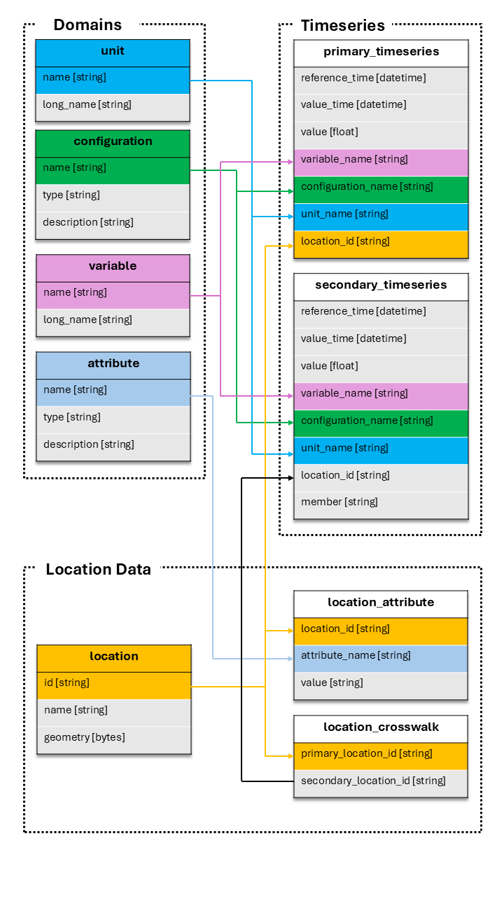
Domain Tables (small reference data, CSV-like):

• units - Measurement units (e.g., “m3/s”, “ft3/s”)

• variables - Variable names (e.g., “streamflow_hourly_inst”)

• configurations - Data source configurations (e.g., “nwm30_retrospective”)

• attributes - Attribute definitions (e.g., “drainage_area”, “ecoregion”)

Location Data:

• locations - Point geometries with IDs (e.g., USGS gage locations)

• location_attributes - Attribute values for each location

• location_crosswalks - Maps primary IDs to secondary IDs (e.g., USGS to NWM)

Timeseries Data:

• primary_timeseries - Observed/reference data (e.g., USGS streamflow)

• secondary_timeseries - Simulated/forecast data (e.g., NWM outputs)

Accessing Tables

There are two ways to access a table:

import teehr

ev = teehr.LocalReadWriteEvaluation(dir_path="./my_eval")

# Method 1: Named property (for standard tables)
locs = ev.locations
pts = ev.primary_timeseries
sts = ev.secondary_timeseries

# Method 2: Generic accessor (for any table)
pts = ev.table("primary_timeseries")
custom = ev.table("my_custom_table")  # User-defined tables

Both methods return a table object with the same methods.

Table Methods Overview

All tables inherit common methods from the BaseTable class:

Output Methods:

• to_sdf() - Return a PySpark DataFrame (lazy)

• to_pandas() - Return a Pandas DataFrame (eager)

• to_geopandas() - Return a GeoPandas GeoDataFrame (eager)

Query Methods:

• filter() - Apply filters

• order_by() - Sort results

• aggregate() - Calculate metrics with grouping

• add_calculated_fields() - Add computed columns

• add_geometry() - Join geometry from locations table

Output Operations:

• write() - Write results to a new table

Table Management:

• is_core_table - True if this table is a built-in TEEHR table

• drop() - Drop a user-created (non-core) table from the catalog

Loading Data

Tables have methods to load data from various file formats. The loading process validates data against the table schema and handles duplicates.

Loading Timeseries Data

Primary and secondary timeseries tables support multiple formats.

From Parquet:

ev.primary_timeseries.load_parquet(
    in_path="./data/observed.parquet",
    field_mapping={
        "datetime": "value_time",
        "discharge": "value",
        "site_no": "location_id"
    },
    constant_field_values={
        "configuration_name": "usgs_observations",
        "variable_name": "streamflow_hourly_inst",
        "unit_name": "m3/s"
    },
    location_id_prefix="usgs"
)

See also: PrimaryTimeseriesTable.load_parquet()

From CSV:

ev.secondary_timeseries.load_csv(
    in_path="./data/forecasts/",
    pattern="**/*.csv",
    field_mapping={
        "forecast_time": "reference_time",
        "valid_time": "value_time",
        "flow": "value"
    },
    constant_field_values={
        "configuration_name": "my_model_v1",
        "variable_name": "streamflow_hourly_inst",
        "unit_name": "m3/s"
    }
)

See also: SecondaryTimeseriesTable.load_csv()

From NetCDF:

ev.secondary_timeseries.load_netcdf(
    in_path="./data/model_output.nc",
    field_mapping={"streamflow": "value"},
    constant_field_values={"configuration_name": "model_run_001"}
)

See also: SecondaryTimeseriesTable.load_netcdf()

From FEWS PI-XML:

ev.primary_timeseries.load_fews_pixml(
    in_path="./data/observed.xml",
    location_id_prefix="fews"
)

See also: PrimaryTimeseriesTable.load_fews_xml()

Loading Parameters

Common parameters for loading methods:

field_mappingdict

Maps source column names to TEEHR schema names:

{"source_col": "teehr_col"}

constant_field_valuesdict

Sets constant values for fields not in source data:

{"configuration_name": "my_config", "unit_name": "m3/s"}

location_id_prefixstr

Prefix added to location IDs for uniqueness:

location_id_prefix="usgs"  # "12345" becomes "usgs-12345"

write_modestr

• "insert" - Insert all rows directly (no duplicate checking, fastest)

• "append" - Add new data, skip duplicates (default)

• "upsert" - Update existing, add new

• "create_or_replace" - Replace entire table

drop_duplicatesbool

Remove duplicate rows during validation (default: True)

Loading Location Data

Load locations from GeoJSON or other spatial formats.

ev.locations.load_spatial(
    in_path="./data/gages.geojson"
)

See also: LocationTable.load_spatial()

Load location attributes.

ev.location_attributes.load_csv(
    in_path="./data/attributes.csv"
)

See also: LocationAttributeTable.load_csv()

Load crosswalks.

ev.location_crosswalks.load_csv(
    in_path="./data/crosswalk.csv",
    field_mapping={
        "usgs_id": "primary_location_id",
        "nwm_id": "secondary_location_id"
    }
)

See also: LocationCrosswalkTable.load_csv()

Loading Domain Data

Domain tables can be populated manually.

# Or add individual records
ev.configurations.add(
    teehr.Configuration(name="my_model", type="model", description="My custom model")
)

See also: ConfigurationTable.add()

Using DataFrames

You can also load from Pandas/GeoPandas DataFrames:

import pandas as pd

df = pd.DataFrame({
    "location_id": ["usgs-01234"],
    "value_time": ["2024-01-01 00:00:00"],
    "value": [100.5],
    "variable_name": ["streamflow_hourly_inst"],
    "unit_name": ["m3 s-1"],
    "configuration_name": ["usgs_observations"]
})

ev.load.dataframe(df=df, table_name="primary_timeseries")

Filtering Data

Filter tables to select specific subsets of data.

SQL String Filters:

ev.primary_timeseries.filter(
    "location_id LIKE 'usgs%'"
).to_sdf().show()

ev.primary_timeseries.filter([
    "value_time > '2024-01-01'",
    "value_time < '2024-02-01'"
]).to_sdf().show()

Dictionary Filters:

ev.primary_timeseries.filter({
    "column": "location_id",
    "operator": "like",
    "value": "usgs%"
}).to_sdf().show()

TableFilter Objects:

from teehr.models.filters import TableFilter
from teehr import Operators as ops

ev.primary_timeseries.filter(
    TableFilter(column="value", operator=ops.gt, value=100)
).to_sdf().show()

See also: PrimaryTimeseriesTable.filter()

Method Chaining

Table methods return self to enable fluent method chaining:

from teehr import RowLevelCalculatedFields as rcf
from teehr import DeterministicMetrics as dm

# Chain multiple operations
result = (
    ev.joined_timeseries_view()
    .filter("primary_location_id LIKE 'usgs%'")
    .add_calculated_fields([rcf.Month(), rcf.WaterYear()])
    .aggregate(
        metrics=[
            dm.KlingGuptaEfficiency(),
            dm.RelativeBias()
        ],
        group_by=["primary_location_id", "month"]
    )
    .order_by(["primary_location_id", "month"])
    .to_pandas()
)

Writing Results

Write query results to new tables:

# Calculate metrics and save to a new table
ev.joined_timeseries_view().aggregate(
    metrics=[dm.KlingGuptaEfficiency()],
    group_by=["primary_location_id", "configuration_name"]
).write("location_metrics")

# Access the new table
metrics_df = ev.table("location_metrics").to_pandas()

You can also write data directly to any warehouse table using ev.write.to_warehouse():

import pandas as pd

df = pd.DataFrame({
    "name": ["m3/s"],
    "long_name": ["Cubic meters per second"]
})

# "insert" — fastest: INSERT INTO with no duplicate checking
ev.write.to_warehouse(source_data=df, table_name="units", write_mode="insert")

# "append" — skip rows that match existing uniqueness fields (default)
ev.write.to_warehouse(source_data=df, table_name="units", write_mode="append")

# "upsert" — update matching rows, insert new ones
ev.write.to_warehouse(source_data=df, table_name="units", write_mode="upsert")

# "overwrite" — replace all data, preserving table history
ev.write.to_warehouse(source_data=df, table_name="units", write_mode="overwrite")

Note

"insert" uses a plain INSERT INTO statement and does not check for duplicates. Use it when you know your data is clean and want maximum throughput. Use "append" (the default) when you want to skip rows that already exist.

See also: Write.to_warehouse()

Deleting Data

There are two equivalent ways to delete rows from a table.

Via a table instance (ev.table().delete() or ev.primary_timeseries.delete()):

# Dry run — preview rows that would be deleted
sdf = ev.table("primary_timeseries").delete(
    filters=["location_id = 'usgs-01234567'"],
    dry_run=True,
)
print(f"Rows to delete: {sdf.count()}")

# Execute deletion on a named table property
count = ev.primary_timeseries.delete(
    filters=["location_id = 'usgs-01234567'"],
)
print(f"Deleted {count} rows.")

# Delete all rows
count = ev.primary_timeseries.delete()

Via the write interface (ev.write.delete_from()):

count = ev.write.delete_from(
    table_name="primary_timeseries",
    filters=["location_id = 'usgs-01234567'"],
)
print(f"Deleted {count} rows.")

Both methods support SQL strings, dicts, and TableFilter objects as filter arguments:

from teehr.models.filters import TableFilter
from teehr import Operators as ops

# Dict filter
count = ev.primary_timeseries.delete(
    filters={"column": "configuration_name", "operator": "=", "value": "old_run"},
)

# TableFilter object
count = ev.primary_timeseries.delete(
    filters=TableFilter(
        column="configuration_name",
        operator=ops.eq,
        value="old_run"
    ),
)

See also:

• BaseTable.delete()

• Write.delete_from()

Dropping Tables

User-created tables (such as materialized views and saved query results) can be dropped when they are no longer needed. Core TEEHR tables (like primary_timeseries and locations) are protected and cannot be dropped.

Use the is_core_table property to check whether a table is a core table before attempting to drop it.

Drop a user-created table via the table instance:

# Write a user-created table
ev.joined_timeseries_view().aggregate(
    metrics=[dm.KlingGuptaEfficiency()],
    group_by=["primary_location_id"]
).write("location_metrics")

# Check whether it's a core table (always False for user-created tables)
ev.table("location_metrics").is_core_table  # False

# Drop the table
ev.table("location_metrics").drop()

Drop a user-created table via the evaluation:

# Convenience method on the Evaluation class
ev.drop_table("location_metrics")

Note

Attempting to drop a core table raises a ValueError:

ev.drop_table("primary_timeseries")  # raises ValueError
# ValueError: Cannot drop core table 'primary_timeseries'. Only user-created
# tables (e.g., materialized views or saved query results) can be dropped.

See also:

• BaseTable.drop()

• BaseTable.is_core_table

• BaseEvaluation.drop_table()

Inspecting Tables

Get information about table contents:

# List all tables
ev.list_tables()

# Get distinct values for a column
ev.primary_timeseries.distinct_values("location_id")

# Get location prefixes
ev.primary_timeseries.distinct_values("location_id", location_prefixes=True)

# View schema (via Spark)
ev.primary_timeseries.to_sdf().printSchema()

Direct SQL Access

For complex queries, use SQL directly:

df = ev.sql("""
    SELECT
        location_id,
        COUNT(*) as record_count,
        MIN(value_time) as first_date,
        MAX(value_time) as last_date
    FROM primary_timeseries
    GROUP BY location_id
""")
df.show()